Employment dropped dramatically in 2008 and 2009. The economic recovery (in gross domestic product) began in June 2009, but it has been an unusually slow recovery, with job growth even slower. As a result, jobs are the biggest issue facing the economy and policymakers.
It is important to understand how job statistics are derived and what that means for public policy.
The Anatomy of the Job Statistics. To-date, the United States has only regained about half of the almost 9 million lost jobs in 2008 and 2009. Job growth has improved recently, but is still below the rate of past recoveries. Consider:
- Payroll employment increased by 171,000 jobs in October and the unemployment rate increased to 7.9 percent, representing 12.3 million people.
- The payroll numbers were revised up by 50,000 in August and by 34,000 in September.
Unemployment averaged below 5 percent before the recession. It peaked at 10 percent in late 2009, and declined to 7.9 percent as of October. It is still about 3 percentage points above what would reasonably be considered normal or full employment.
The situation, however, is worse than these numbers portray. Not only is unemployment high as a percent of the labor force, but the labor force itself has been shrinking as job seekers give up and drop out. Indeed, labor force participation (job seekers and the employed) has declined from 66 percent before the recession to 63.8 percent. Moreover, employment, as a percent of the population, has declined from over 63 percent before the recession to 58.8 percent in October.
These numbers are estimates based on samples, which make them subject to sampling error. The payroll number comes from reports submitted by 141,000 business establishments and government entities representing about 486,000 workers. Statistically, at the 90 percent confidence level, the “true” payroll change is the estimated number plus or minus 100,000. In October, that is between 71,000 and 271,000. A larger sample size would narrow that range by reducing the sampling error.
The unemployment rate is derived from a separate household survey, which has an even smaller sample size and a wider confidence range. The survey of 60,000 households is done mostly by phone. Respondents answer questions like, are you currently employed? If yes, the responder is counted as employed. If no, the responder is asked if they have actively sought employment in the past 6 weeks. If yes, the respondent is considered in the labor force, but unemployed. If no, they are considered outside the labor force, but not unemployed.
 Because the household survey’s sample size is smaller than the establishment survey, its confidence range is larger. At the 90 percent confidence level, the “true” number of unemployed persons is the estimated number plus or minus 280,000, and the “true” unemployment rate is the estimated rate plus or minus 1.9 percentage points. Thus, the estimated unemployment rate of 7.9 percent in October means that the “true” rate was between 6 percent and 9.8 percent.
The duration of unemployment has been longer than in past recoveries. In October, 5 million people had been unemployed over 27 weeks — just over 40 percent of the 12.3 million people unemployed. The length of the work week was 34.4 hours, while average hourly earnings were $23.58, or $811.15 per week.
How the Statistics Are Broken Down. The unemployment stats are broken down several ways. For example, unemployment rates are higher for minorities than non-minorities, and they are higher for teenagers than for adults. Indeed:
- The teenage unemployment (16 to 19 year olds) was 23.7 percent in October.
- The rates for adult men and adult women (20 years and over) were 7.3 and 7.2 percent, respectively.
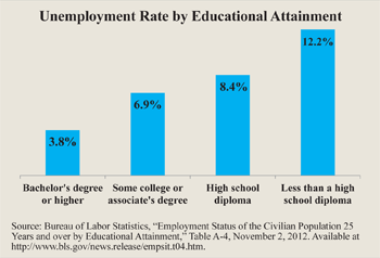
The unemployment breakdown most relevant to those entering the job market is by education. Consider [see the figure]:
- Compared to an overall average of 7.9 percent, unemployment was 3.8 percent for bachelor’s degrees or higher, and 6.9 percent for some college or an associate’s degree.
- It was 8.4 percent for high school graduates with no college.
- And the rate was 12.2 percent for those with less than a high school diploma.
The message here: stay in school.
Policy Implications. Higher levels of employment and lower levels of unemployment are highly desirable. The role of government is to promote a healthy economic environment so that the demand for workers, primarily by the private sector, will accommodate all those who are able, willing and want to work. But creating jobs for sake of it is not a proper goal of government policy. Indeed, jobs should not be the primary goal of public policy, but the by-product of other desirable goals.
Governments may save jobs by discouraging new technology. Think of all the elevator and telephone operators we have lost in recent decades, but we are better off because they moved on to more needed jobs. Think of all the farm jobs lost to tractors and other farm equipment, and all the factory jobs lost to labor-saving technology.
This sounds counterintuitive, but you can probably measure national economic progress more by jobs destroyed, than by jobs created. It once took 90 percent of our population to grow our food. It now takes 2 percent. Do we bemoan the farm jobs lost or celebrate the productivity gains that they represent?
Government should not protect jobs made obsolete or unproductive by technology, or by creating or tolerating inefficiencies (for example, teachers’ unions). Instead it should encourage a vigorous private sector to be able to absorb those caught up in creative destruction.
Ironically, wages and jobs depend on labor productivity, which is a function largely of the capital base labor has to work with. Government should not discourage capital formation through excessive regulation or taxation, even if encouraged to do so by misguided labor organizations.
Robert McTeer is a distinguished fellow with the National Center for Policy Analysis.