Social Security Reform: Responding to the Critics

Critics of President Bush’s Social Security reform proposal have used findings by Robert Shiller, professor of economics at Yale University, to suggest that many workers will lose money if they open personal retirement accounts (PRAs), which are a key component of the president’s reform approach.

Under a reformed system, American workers would release the government from the obligation to pay some of their expected retirement benefits in exchange for the opportunity to invest some of their payroll taxes through personal accounts. The amount of the reduction is based on what the personal account is estimated to grow to if it were invested entirely in government bonds. The monthly life annuity that could be purchased with this hypothetical accumulation is called the “benefit offset.”

If the annuity generated from a personal account is greater than the benefit offset, the worker gains from owning a PRA. If the account balance is less than the benefit offset, a worker would have been better off without the account.

Shiller measures how workers would fare under the president’s approach using financial market returns from 1871 to 2004 to construct 91 overlapping 44-year time periods. But instead of using the actual return on government bonds over these periods to determine the benefit offset rate, he uses a higher fixed real rate of 3 percent, which is the projected future government borrowing rate. Under these assumptions, in one-third of these time periods workers would have been worse off than if they had not invested at all.

However, as Shiller notes, the 3 percent offset rate is too high, and he suggests using a market return. Using the actual, historical bond rate of return to calculate the benefit offset, we repeated the simulations. The result provides a picture of how workers would fare under the president’s approach, if it were to incorporate the realized government borrowing rate. Based on the historical data we found that:

• Workers with balanced portfolios of stocks and bonds exceed the break-even point in all of the simulations.
• Workers who invest in a lifecycle fund suggested by Shiller will experience a net gain (personal account balance minus the benefit offset) of $15,830 to $102,031, with a real internal rate of return ranging from 1.57 percent to 4.68 percent, depending on the simulation.
• If a worker instead invests in a more aggressive lifecycle fund, the net gain is $50,533 in the worst scenario and $248,400 in the best scenario.
• Based on the historical data, some workers’ net gain would have exceeded the benefit offset amount by more than two-and-a-half times.

There are two additional features that can be employed to protect workers from the ups and downs of the market. First, to avoid the pitfall of having to purchase an annuity in a down market (for example, requiring people to annuitize their personal accounts on their 65th birthday), workers could annuitize their PRAs over several years. In addition, workers could be allowed to purchase an annuity as soon as their accounts are large enough to support a specified pension, regardless of their age.

Second, workers who invest in a balanced portfolio of stocks and bonds can be assured they will receive at least the reformed Social Security benefit by setting the actual offset to either the PRA balance or the benefit offset amount, whichever is less. That is, with this provision, a worker who invests in a diversified portfolio will never be worse off for having opted for a PRA.

“President Bush has proposed allowing workers to prefund some Social Security benefits by saving in personal retirement accounts (PRAs).”

President Bush’s push to reform Social Security has many critics. The president has proposed allowing workers to prepay a portion of their retirement benefits with personal retirement accounts (PRAs). He also supports changing the way benefits are calculated in order to restrain their future growth. Some critics of the president’s approach have used findings by Robert Shiller, professor of economics at Yale University, to take issue with a particular feature of Bush-style PRAs called the “benefit offset.” Shiller’s findings have been used to suggest that this provision will cause many workers with PRAs to fare worse than if they had not had these accounts.

This paper examines the critics’ concerns and finds that many of them are addressed by an alternative benefit offset. Shiller noted in his paper that “the 3% real offset rate appears to be too high, and if the program is instituted, it should be done with a lower rate.…Better yet, the offset could be cumulated at a market rate. The offset could be calculated as the terminal value of the contributions brought to the final date using actual U.S. Treasury Inflation Protected Security (TIPS) yields of the appropriate maturity.” In this paper, we do just that by using a benefit offset based on the realized government borrowing rate. With such a rate, most workers with a personal account will retire with higher benefits than they would have without the account.

“To pay benefits in 2017, and every year thereafter, Social Security will require transfers from the rest of the federal budget.”

President Bush has made reforming Social Security a top priority. Students of Social Security know the program’s tax revenues will fall short of its costs beginning in 2017, and the gap between tax revenues and benefit payments grows each year thereafter. Based on past surpluses that have been credited to the Social Security Trust Fund and projected surpluses until 2017, the system has dedicated funding until 2041. However, drawing on these dedicated funds implies general revenue transfers that will require the federal government to reduce spending elsewhere, raise taxes and/or increase borrowing.

The President’s Plan. To close the funding gap, President Bush has outlined a plan that incorporates paying for a portion of future benefits through individual investments. While the details of the president’s approach have yet to be determined, it appears the reform has two major components: 1) reduce the growth in initial benefit payments by changing the indexing formula from one based exclusively on wage growth to one based on progressive price indexation, and 2) establish PRAs for younger workers. The two reforms combined will produce total benefits for all income groups that are similar to currently scheduled benefits, and produce potentially much higher benefits for lower-income workers. ¹

Progressive Price Indexing. Currently, Social Security calculates benefits for all new retirees by averaging a worker’s 35 highest-earning years and putting his or her average wage-indexed earnings through a benefit formula. The worker’s earnings are adjusted, or indexed, to the annual increase in average wages nationwide. Given that wages typically rise faster than prices, the real purchasing power of the average Social Security benefit paid to new retirees will increase more than 60 percent over the next 50 years while maintaining the current replacement rate of about 41 percent of preretirement earnings.

“Robert Pozen has proposed indexing benefits for higher income workers to prices rather than wages.”

Unfortunately, under current law, Social Security cannot afford to pay what is scheduled. Robert Pozen, a member of President Bush’s 2001 Commission to Strengthen Social Security, has proposed progressive indexing as part of a reform that results in a sustainable program in the long run. Under the Pozen approach: ²

• Benefit calculations would not change for current retirees, near retirees or income earners in the bottom 30 percent of lifetime earnings (about $25,000 a year or less). These workers would receive the same Social Security benefits scheduled under current law.
• However, starting in 2012, initial benefits for the highest earners would be determined by the growth in prices, rather than wages.
• The growth each year in initial benefits for workers between $25,000 and the maximum would be set by a progressive mix of prices and wages.

Thus, Social Security benefits of lower earning workers would be the same as those currently scheduled, while benefits for the highest earners would grow with inflation but not reap the additional boost from real wage growth.

“Progressive price indexing can be combined with PRAs funded by 4 percentage points of workers’ payroll taxes.”

Personal Retirement Accounts. The current outline of the president’s proposal also calls for depositing 4 percentage points of a worker’s payroll taxes into a personal account — up to $1,000 annually — starting in 2009. After 2009, the maximum contribution would rise each year by $100 plus wage growth, ultimately resulting in 4 percent accounts for all workers. At retirement, a worker’s account balance would be used to purchase an inflation-protected lifetime annuity, which would supplement the new price-indexed benefit from the traditional Social Security system.

Under current law, workers remit their Social Security payroll taxes to the federal government in exchange for a retirement pension, survivors insurance and insurance against disability. Under personal account reforms, workers would release the government from the obligation to pay some of their expected retirement benefits in exchange for the opportunity to redirect some of their payroll taxes to personal accounts.

The Benefit Offset. Most PRA plans propose to accumulate the worker’s personal account contributions in a shadow account by applying a specified interest rate for each pre-retirement year. The monthly life annuity that could be purchased with this hypothetical accumulation is the benefit offset. A worker’s retirement pension would be determined by subtracting the offset amount from his price-indexed benefit and adding his personal account annuity:

Thus, if a worker’s account earns a higher rate of return than the benefit offset amount, he will earn a higher total benefit than if he did not have the account. By contrast, if the worker’s rate of return falls below the offset, he would have been better off without the account.

“As the PRAs grow, the benefit paid by Social Security is reduced (the benefit offset).”

Looked at another way, the benefit offset provides a way to repay taxpayers for the current costs of moving to the new system. From this perspective, the offset is simply a repayment to the government by personal account holders of the money the government loaned them to invest in the stock and bond market. At retirement, workers must repay the loan with interest. ³

If the benefit offset rate is set at the government’s borrowing rate, the effect on the government’s finances is neutral, assuming the government borrows the funds that are ultimately deposited in the accounts. The combination of the new current (explicit) debt and the ultimate offset repays all the borrowing with interest and thus implies no net change in the government’s total debt.

The remainder of this paper examines the likelihood that workers who open a PRA will lose money. That is, we estimate the chance that a worker’s personal account annuity is less than the benefit offset annuity. If so, the new price-indexed benefit would be reduced by the difference and would be smaller than if the worker had not opted for the account.

Criticisms of the Plan Based on Shiller’s Findings. The president’s plan has been criticized in several ways. First, as stated above, some worry that many workers will receive lower benefits because their total account return will fall below the government’s borrowing rate. Second, there is a concern that workers’ investments will frequently earn less than the government borrowing rate.

Shiller raises both issues in a recent study. ⁴ He assumes that workers invest in “lifecycle accounts,” as has been suggested by the president. These accounts are designed to gradually and automatically reduce the percentage of a portfolio invested in stocks as workers age, allocating more to stocks when workers are young and more to bonds as they near retirement. ⁵ Using actual historical stock returns dating back to 1871, Shiller finds that 32 percent of the time an account patterned after the president’s will produce returns that fall below the 3 percent assumed for the benefit offset. This implies that one-third of the time new retirees would have to subtract an additional amount from their price-indexed Social Security benefits; thus, they would have lower benefits than if they had not opened an account. Using a lower rate of return on stocks to reflect reduced expectations about future returns, Shiller finds that 71 percent of the lifecycle portfolios fall below the 3 percent break-even point.

An Alternative Benefit Offset Rate. As Shiller noted, the 3 percent benefit offset rate is too high. As a result, it pushes many more portfolios below the break-even point than if a lower return, such as the actual historical government bond rate of return, had been used.

“The size of the benefit offset account used here is determined by the realized rate of interest paid on government bonds.”

As evaluated by the Social Security Actuaries, the personal account proposed by the Bush Administration uses the prospective government borrowing rate as the rate of return for determining the benefit offset. ⁶ However, it is more appropriate to use realized government bond returns — not a fixed rate (for example, 3 percent) — when evaluating the likelihood that a worker’s personal account will accumulate less than the benefit offset. ⁷ Specifically, if the purpose of the benefit offset is to repay the funds provided to the worker by the government, then the realized bond rate over the worker’s life is the appropriate offset rate. ⁸

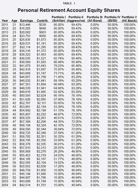
In what follows, we replicate Shiller’s simulations, but with an important difference: instead of using a fixed 3 percent rate of return to calculate the benefit offset, we use the realized return on government bonds. We also evaluate five portfolios — two lifecycle portfolios and three constant allocation portfolios — using several different methods.

Selecting Portfolios . We consider five asset allocations that differ in the ratio of stocks to bonds. Table I presents the proportion of stock at each age for the five portfolios.

• Lifecycle Fund Based on Shiller: Invested 85 percent in equities through age 29; it gradually falls to 15 percent in equities by age 60. This reflects the allocation rule considered by Shiller. ⁹
• More Aggressive Lifecycle Fund: Invested 89 percent in equities through age 29; it falls in six 5-year steps to 47 percent in equities by age 60. The equity to bond allocation is based on the Fidelity Freedom series fund as of December 31, 2004.
• All Bond Fund: Invested 100 percent in bonds; 50 percent in long-term government bonds and 50 percent invested at the money-market rate.
• 50/50 Fund: Fixed at 50 percent equities, 30 percent corporate bonds and 20 percent Treasury bonds; it does not vary over workers’ lifecycles. This corresponds to the featured portfolio considered by the 2001 President’s Commission to Strengthen Social Security. ¹⁰
• All Stock Fund: Invested 100 percent in equities throughout the workers’ years in the labor force.

Using Lifecycle Funds . Lifecycle portfolios are often mentioned as a way to address the perceived risks of investing in the stock market. Lifecycle portfolios are funds that automatically reduce the level of risk as the owner ages by gradually reducing the level of stock and increasing the level of bonds over time. The idea is that the portfolio should become more conservative as individuals near retirement. However, lifecycle portfolios have been available for only a few years. It is difficult to evaluate their performance based on the few existing funds over such a short period of time.

“Returns for five hypothetical investment portfolios were calculated for 91 overlapping 44-year periods.”

Instead, we examine the historical performance of the U.S. stock and bond markets since 1871 and create two hypothetical portfolios that follow the allocation used by Shiller and the more aggressive allocation identified above. ¹¹ Returns on equities, six-month money market rates and long term government bond returns (all adjusted for inflation) are used to construct returns on our two lifetime portfolios and the other three fixed allocation portfolios.

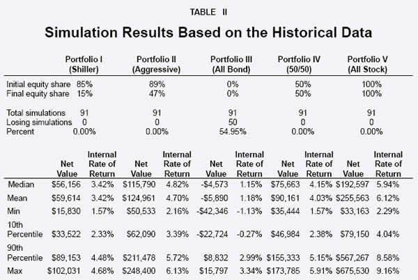
How often will the rate of return on a worker’s PRA fail to reach the break-even point (the benefit offset amount)? Or, how frequently can workers expect a net loss?

Imagine a worker who joins the workforce in 2011 at age 21, opens a PRA and retires after working 44 years. The hypothetical worker’s earnings and contributions to a personal account are presented in Table I. Applying this earnings profile to all 91 overlapping 44-year historical periods we calculate the frequency with which the personal account returns, based on the five portfolios, accumulate less than the benefit offset. Administrative fees are assumed to be 0.3 percentage points. Table II and Figure I summarize the results for the five portfolios. ¹²

The upper panel of Table II identifies the frequency with which the five portfolios do not achieve the rate of return used to calculate the benefit offset (which is the realized long-term government bond rate). At the end of the contribution period, if the net value of the personal account — the account balance minus the benefit offset — is negative, then the account is designated as suffering a loss.

“Historical data shows all the investment portfolios (except the all bond fund) will have a higher return than the benefit offset account.”

As can be seen in both the figure and the table, all portfolios perform better than the benefit offset in all 91 simulations with the exception of the “All Bond Fund” (50 percent in long-term government bonds and 50 percent invested at the money-market rate). A worker who held the all bond portfolio in his personal account would do worse than the benefit offset slightly more than half the time. Workers who held any of the other three portfolios would have benefited from owning a personal account because their account would be worth more than the benefit offset when they retired.

How much better would these workers have fared? The lower panel of Table II contains a summary of the net values and the associated internal rates of return for each of the five portfolios. The portfolios’ net values are equal to the difference between the total personal account accumulation minus the benefit offset. The personal account is always positive after the benefit offset — meaning it earns a return greater than the benefit offset rate — except for the all-bond portfolio. According to the table:

• Workers who invested in the “Lifecycle Fund based on Shiller,” would experience a net gain of $15,830 to $102,031, with an internal rate of return ranging from 1.57 percent to 4.68 percent.
• If the worker invested in the “More Aggressive Lifecycle Fund,” the account would end up with a net gain of $50,533 in the worst scenario — the 1877-1920 contribution period — and $248,400 in the best scenario, for the 1922-1965 contribution period; the average return is 4.7 percent after expenses.

The last two columns report the net values and internal rates of return produced by the “50/50 Fund” and the “All Stock Fund.” As shown in Figure I, the all-stock portfolio out-performed the other portfolios in almost all years. Out of 91 simulations, the all-stock portfolio fell short of the more aggressive lifecycle fund in only five cases, and all by relatively small margins.

“The all stock portfolio yields the highest return; all bond investments yield the lowest returns.”

These results — using realized government bond rates to calculate the benefit offset — are a striking contrast to Shiller’s findings based on the fixed 3 percent benefit offset. Recall Shiller found that in 32 percent of the cases using his baseline lifecycle account, the personal account fell short of the benefit offset amount. By contrast, using the realized government bond return to determine the benefit offset, this same account never falls short. ¹³

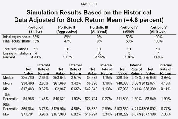
“Many argue that the performance of the U.S. stock market in the past century may not be repeated in the future.”

Shiller also considered the effects on his results if the equity premium were to decline, meaning he assumed a lower estimated return for stocks. Predicting future long-term stock returns is extremely difficult. Often past experience is used as a guide to future expectations. But many argue that the performance of the U.S. stock market in the past century may not be repeated in the future. Due to demographic changes, the capital-to-labor ratio will rise and returns on domestic capital may decline, which in turn may lower long-run stock returns. Sometimes analysts use lower expected equity premiums, among other tools, to account for these effects and reduce forecasts of future stock returns. However, other factors will likely mitigate these effects. For example, the integrated global capital market will continue to be affected by the increasing demand for capital from China, India and many other developing nations in their move toward greater industrialization.

To investigate the effects of declines in equity returns, we repeat the simulation exercises from the last section using an adjusted stock return series. Specifically, we reduce all historical stock returns by a fixed amount such that the geometric average return of the adjusted series is 4.8 percent. The adjusted estimates using the 4.8 percent average return are presented in Table III and Figure II. The choice of a 4.8 average return follows Shiller. ¹⁴

With these mean-return adjustments, we assume that stock market volatility remains unchanged. We also implicitly assume that the bond market volatility and returns are unchanged from the historical levels. Thus, this exercise essentially represents a reduction in the equity premium with no associated reduction in risk. We discuss the implications of this assumption further below.

Note that the results for the all bond fund remain unchanged. For the other four portfolios, which include equities, there is a small probability that the portfolio will fall below the benefit offset threshold. As expected, a comparison of Figures I and II shows the returns on portfolios with equities decline as a result of the assumed reduction in the equity premium. Remember Shiller projected an alarming frequency of outcomes falling below the break-even point, based on a static 3 percent benefit offset rate. By contrast, simulations using the realized rate of return on government bonds produces few outcomes below the benefit offset amount. For example, the lifecycle fund using Shiller’s base case allocation produced only 4 such simulations out of 91, or 4.4 percent, whereas Shiller reported 65 to 71 percent.

“Even using lower returns, the stock portfolio still outperforms the benefit offset rate.”

The same holds for the other portfolios. Clearly, using a benefit offset rate based on the realized government borrowing rate eliminates much of the concern over the return on workers’ accounts falling below the benefit offset rate. In short, based on historical data, workers would have seen their personal accounts outperform the benefit offset account almost all the time.

One of the shortcomings of using historical data is the fact that there are few independent simulation periods. However, there are several techniques that allow researchers to simulate data and in a sense examine more time periods. The Appendix details our simulation results, but they are summarized here briefly.

“Our assumptions are conservative.”

The simulation results based on 1,000 independent 44-year investment periods are consistent with the results based on the historical period, but the percentage of simulations in which the portfolios perform worse than the benefit offset threshold is slightly higher. We consider one-year and five-year sampling blocks. The first assumes that the year-to-year ordering of the sampled data is random, while the second attempts to capture the possibility of mean reversion over a longer period. The longer block reduces the rate of portfolios falling below the benefit offset. For the two lifecycle portfolios, the personal account returns fall below the benefit offset about 6 percent to 7 percent of the time when the simulated data is drawn from the unadjusted historical data.

When the simulated data is drawn from data we have adjusted to reflect a possible reduction in the equity premium, the failure rate rises.

However, we caution that a reduction in the equity premium should carry with it a reduction in the variability of the stock returns. Because our simulations in the Appendix and in the previous section did not include a reduction in the variability of stock returns, our estimates using adjusted stock return data probably overestimate the cases where accounts fall short of the benefit offset.

One way to protect workers against the downside risk is to set the benefit offset to the minimum of the hypothetical account accumulation using the realized government borrowing rate and the PRA. With such a provision, any worker who opens a PRA and invests in a balanced portfolio of stocks and bonds will receive at least the price-indexed Social Security benefit. If this provision is offered, the simulations above and in the Appendix provide estimates of the frequency with which the government receives less than the amount borrowed. Clearly, this provision is not costless to the government, and ultimately to taxpayers. However, this assurance can be thought of as compensation for the reduction in benefits through progressive price indexation.

The government could guarantee this minimum benefit to any worker who invests in a diversified portfolio and does not meet the benefit offset threshold. The portfolio that is assured can be the default option for workers who open a personal account and would have a prescribed portfolio allocation throughout the workers’ lifecycle. Of course, workers who wish to invest more aggressively could do so, but risk the losses that come with the opportunity for higher returns.

“The government could guarantee a minimum benefit to low income workers.”

Since the historical data produces few outcomes below the break-even point and the rate of portfolios falling below the break-even point with the simulated data is not excessive, some suggest that guaranteeing the price-indexed benefit would be inexpensive. Others have been much more cautious. ¹⁵ Regardless of how one looks at the historical and simulated evidence, the discussion of guarantees ignores two important facts. First, current Social Security benefits are not (and never have been) guaranteed. Second, even if current Social Security benefits were guaranteed, they would have the same implicit costs as the guarantees that are discussed in the context of personal accounts.

This downside risk protection would definitely make the reformed system superior to the current system for low income workers in the event that the reformed system combines personal accounts with progressive price indexing. All workers whose lifetime average earnings are less than the earnings level where indexing starts only have the upside potential of the amount by which their personal account exceeds the benefit offset.

PRA holders will likely be required to purchase an annuity with their account balance at retirement. The annuity will provide a monthly benefit payment for life that would be combined with the price-indexed benefit the worker receives from the traditional taxpayer-funded Social Security system.

“Workers could gradually purchase retirement annuities with their PRAs.”

Features can be built into the system to help retirees avoid annuitizing their entire account accumulation at the bottom of a down market. For example, workers could annuitize their personal account benefit over several years. Laurence Kotlikoff has suggested gradually annuitizing each worker’s personal account between the ages of 57 and 67. ¹⁶ Coupling the gradual sale of personal account assets with a benefit offset threshold that is adjusted throughout the process would reduce the frequency of failures.

Another way would be to allow workers with accounts large enough to provide a specified minimum benefit (when combined with their benefits from the traditional Social Security system) to annuitize their accounts at any time, as is the case in Chile. ¹⁷

As this paper demonstrates, a benefit offset rate that tracks the realized rate of return on government bonds, rather than being set at a static rate, will increase the likelihood that workers’ returns on their personal retirement accounts will outpace the benefit offset.

“Using the realized government borrowing rate is in the spirit of the rationale for the benefit offset.”

This paper addresses the frequency with which PRA accumulations fall short of those that would result from investing in a pure government bond account which represents the benefit offset amount. We follow Shiller’s recommendation that the benefit offset rate be computed using a market rate of return rather than a fixed 3 percent return. ¹⁸ Our treatment using the realized government borrowing rate is in the spirit of the rationale for the benefit offset, which is to repay the government for the loan provided to workers. We also report on a more aggressive life-cycle investment strategy and provide estimates based on simulated data.

In contrast to Shiller’s findings we find that:

• None of the portfolios which include equities fall short of the benefit offset amount when we use unadjusted historical data, and thus provide net benefits to retirees.
• Even when the historical stock returns are adjusted downward by reducing the average return to 4.8 percent, reflecting a substantial decline in the equity premium, we find that at most, 7.7 percent of the 91 overlapping historical time periods would produce negative net benefits.

NOTE: Nothing written here should be construed as necessarily reflecting the views of the National Center for Policy Analysis or as an attempt to aid or hinder the passage of any bill before Congress.

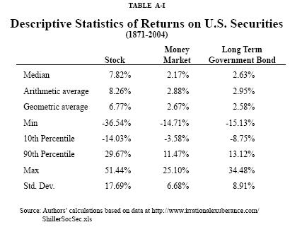
This paper uses three types of security returns to construct returns on lifetime portfolios: equity returns, six-month money market rates and long term government bond returns (all in real terms deflated by consumer price index. Table A-I provides some descriptive statistics. For the 134-year period, the geometric average return of stocks was 6.77 percent, higher than those of short term money market (2.67 percent) and long term bonds (2.58 percent). Not surprisingly, the volatility in the stock market is higher than that of the two lower return securities. Note that even the six-month money market rate is not risk-free. It has a standard deviation of 6.68 percent, which is a measure of variation around the average return. The long-term government bond’s real return is more volatile. The limitation of the empirical return data is obvious: although it spans a period of 134 years, it contains only three independent 44-year periods, the number of years the hypothetical worker is in the work force. It is a small sample from a statistical viewpoint. Therefore, subsequent to the estimates based on the historical and adjusted historical data, the five portfolios are also evaluated using simulated data.

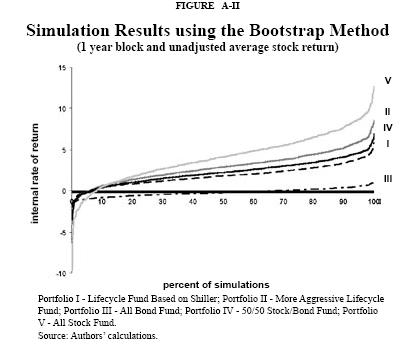
Results Based on Bootstrap Method. In this section we simulate the stock and bond returns using estimates based on the historical data. We simulate 1,000 series of 44 years worth of bond and stock returns following the using a method known as the bootstrap method. The “bootstrap” method relies on the realized historical distributions of stock and bond returns to generate the simulation data. This method can be thought of as sampling from the sets of historical bond and stock returns. It is as if each of the 134 historical sets of bond, stock, and money market returns are represented on separate slips of paper in an urn. Slips of paper are drawn from the urn (and replaced) 1,000 times to produce the results presented in Table A-II and in Figure A-I.

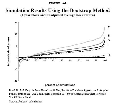
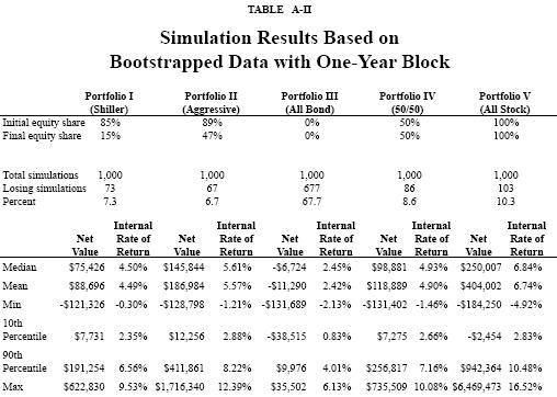
The results summarized in Table A-II indicate that the simulated data produce higher failure rates than did the actual historical data summarized in Table A-I. Note that for the four portfolios which include some stocks, the probability of a losing simulation ranges from a low of 6.7 percent for the more aggressive lifecycle portfolio to a high of just over 10 percent for the all stock portfolio. Figure A-I presents an alternative way of summarizing the simulation results for all five portfolios. For each of the 1,000 simulations the benefit offset internal rate of return, the return associated with a 100 percent government bond portfolio, is subtracted from each of the five the portfolio returns. Positive values represent PRA accumulations in excess of the benefit offset account accumulation (winning simulations) while negative values represent PRA accumulations less that the benefit offset rate (losing simulations). As depicted, and as was presented in Table A-II, less than 10 percent of the independent, non-overlapping simulations based on portfolios that include equities result in losing outcomes.These results should be interpreted slightly differently than the results presented in Table II. Recall that the results in Table II represent 91 overlapping 44 year periods, while these results represent 1,000 simulated independent periods. Also, by drawing single years or sets of stock, bond, and money market returns and arranging them randomly may not represent the true data generating process. However, it serves as a benchmark way of simulating the data by assuming that the ordering of returns is random.

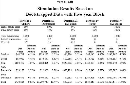
Results Based on Bootstrap Method with Five-Year Block. If returns on financial instruments are mean-reverting; that is, if returns have a natural tendency to move towards the mean over extended periods, then the assumption of random ordering may result in a higher failure rate. Table A-III and Figure A-II summarize a simulation in which the order is maintained for five-year blocks of data. Five-year blocks are chosen given that the average business cycle spans approximately five years. In this simulation, beginning years of the five-year block are sampled with replacement from the first 130 years of the historical period. In this way a 44 year period is constructed after making 9 draws. As the summary statistics indicate, this procedure produces similar distributional properties for the rates of return, but the failure rates decline for all of the portfolios that include equities. The percentages of losing simulations range from 5.7 to 8.1 percent for an average reduction in failure rates of 1.8 percent­age points relative to results obtained with the random ordering assumption. Again the more aggressive lifecycle portfolio had the fewest simulations where returns fell below the benefit offset rate.

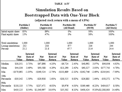
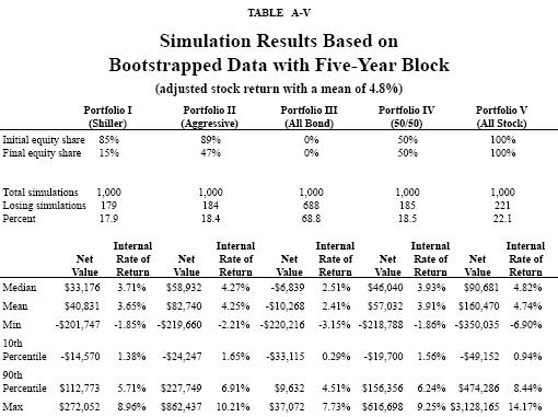
Tables A-IV and A-V summarize simulation results for which the average stock return has been reduced to 4.8 percent and the sampling block is 1 and 5 years, respectively. As with the results based on the adjusted historical data summarized in Table III, no attempt to reduce the variance in the stock returns has been made. This assumption produces an upper-bound failure rate given that the variance in equity returns would be expected to fall with a compression in the equity premium. As Table A-IV indicates, if the ordering of returns is random in the simulation, the failure rates range from 21.2 to 24.4 percent for the portfolios that include stock. The corresponding failure rates range from 17.9 to 22.1 percent when 5-year blocks of returns are sampled. ¹⁹

1. See Andrew J. Rettenmaier and Thomas R. Saving, “Social Security and Progressive Indexing,” National Center for Policy Analysis, Brief Analysis No. 520, July 11, 2005.
2. See the solvency memorandum from Stephen C. Goss, Chief Actuary of Social Security, to Bob Pozen dated February 10, 2005 for further details and for an evaluation of the proposal. Note that Pozen’s plan coupled the particular adjustment to the benefit formula outlined with accounts equal to 2 percent of earnings. However, the benefit offsets are conceptually the same regardless of the account size.
3. Another vantage point from which to view the transaction is that of the workers. In effect they have an arrangement with the government in which they agree to pay taxes in exchange for a retirement pension and an insurance policy. In this view, workers are the lenders rather than the government. For the opportunity to redirect their taxes to personal retirement accounts, workers must relinquish some of their benefits that they would otherwise expect from the government. With this understanding, the benefit offset rate is not the government borrowing rate but rather the implicit return to Social Security. This return could be higher or lower than the government borrowing rate and future rates are subject to legislative reforms.
4. Robert J. Shiller, “”>The Life-Cycle Personal Accounts Proposal for Social Security: An Evaluation,” March 2005. Web publication.
5. In an attempt to address the perceived risks embodied in investing in the stock market, an oft-mentioned investment strategy uses lifecycle portfolios (also known as funds of funds, allocation funds and pre-mixed portfolios.) A “lifecycle account” invests in a pre-mixed portfolio of stocks and bonds, and automatically adjusts the level of risk as the worker ages, primarily by changing the allocations of equities and bonds. An example of a lifecycle account is the Vanguard Total Retirement 2045 Fund. The fund is targeted toward a person retiring in 2045; the fund invests almost completely in stocks, but gradually and automatically shifts to almost all bonds by 2045. The mix of stocks and bonds — and the rate of the replacement of one with the other — has a dramatic effect on the fund’s returns.
6. See solvency memorandum from Stephen C. Goss to Charles P. Blahous, February 3, 2005.
7. See the solvency memorandum from Chris Chaplain and Alice H. Wade to Stephen C. Goss, Chief Actuary of Social Security, November 18, 2003, which evaluates a proposal introduced by Sen. Lindsey Graham for a proposed benefit offset rate equal to the realized long term bond rate less 0.3 percentage points.
8. Note that the 2005 Social Security Trustees Report projects the government’s borrowing rate — the real rate of return on government bonds — will average 3 percent above inflation. This rate is appropriate for static projections of the benefit offset, but it is not the appropriate rate for performing stochastic simulations if the intent of the benefit offset is to repay additional government borrowing during a worker’s lifetime.
9. Robert J. Shiller, “The Life-Cycle Personal Accounts Proposal for Social Security: An Evaluation,” March 2005.
10. President’s Commission to Strengthen Social Security, Strengthening Social Security and Creating Personal Wealth for All Americans, 2001.
11. Market returns on equity are represented by total returns on Standard & Poors 500 stocks including both capital appreciation and dividend income. The historical stock and money market and long term government bond return series are compiled by Robert J. Shiller, “The Life-Cycle Personal Accounts Proposal for Social Security: An Evaluation,” March 2005.
12. For the full discussion of assumptions and for additional findings see the Appendix.
13. Note that the internal rates of return presented in Table II are essentially identical to the results Table 3 of Robert J. Shiller, “The Life-Cycle Personal Accounts Proposal for Social Security: An Evaluation,” March 2005.
14. Ibid.
15. See Campbell and Feldstein, eds., Risk Aspects of Investment-Based Social Security Reform (Chicago: University of Chicago Press, 2001), for a collection of papers that discuss in detail how to address risk in Social Security reforms involving personal investment accounts.
16. Laurence Kotlikoff, “Fixing Social Security for Good” presented at the University of Maryland on September 13, 2003.
17. See Estelle James, “Private Pension Annuities in Chile,” National Center for Policy Analysis, Policy Report No. 271, December 2004.
18. Robert J. Shiller “The Life-Cycle Personal Accounts Proposal for Social Security: An Evaluation,” March 2005.
19. We also conducted additional simulations based on an alternative bootstrapping procedure, simulations which assume that returns are distributed log normally, and a simulation that allows for variable wages over the investment period. Those results appear in Rettenmaier and Wang (2005).

Dr. Andrew J. Rettenmaier is the Executive Associate Director at the Private Enterprise Research Center at Texas A&M University. His primary research areas are labor economics and public policy economics with an emphasis on Medicare and Social Security. Dr. Rettenmaier and the Center’s Director, Thomas R. Saving, have presented their Medicare reform proposal to U.S. Senate Subcommittees and to the National Bipartisan Commission on the Future of Medicare. Their proposal has also been featured in the Wall Street Journal, New England Journal of Medicine, Houston Chronicle and Dallas Morning News. Dr. Rettenmaier is the co-principal investigator on several research grants and also serves as the editor of the Center’s two newsletters, PERCspectives on Policy and PERCspectives. He is coauthor of a book on Medicare, The Economics of Medicare Reform (Kalamazoo, Mich.: W.E. Upjohn Institute for Employment Research, 2000) and an editor of Medicare Reform: Issues and Answers (University of Chicago Press, 1999). Dr. Rettenmaier is a senior fellow with the National Center for Policy Analysis.

Dr. Zijun Wang is an Assistant Research Scientist of the Private Enterprise Research Center at Texas A&M University. His primary research interests are econometric forecasting, empirical consumption analysis and health economics. Dr. Wang has published in the Journal of Forecasting and has presented his research on stock market volatility at an international conference. He has served as a referee for Economic Inquiry. Before coming to the United States Dr. Wang published several papers on the Chinese economy, and is the co-author of Road Toward Market Economy, Xinhua Press House, Beijing, 1993. Dr. Wang has worked extensively on Medicare and Social Security research since he joined the Private Enterprise Research Center.